
Neural networks are a type of machine learning algorithm inspired by the way the human brain works. They are composed of layers of interconnected "neurons" that can learn to recognize patterns in data. Each neuron takes in input values, performs some calculations, and passes its output to the next layer of neurons until a final output is produced. The process of training a neural network involves adjusting the strength of connections between neurons so that the network can accurately classify or predict outcomes based on input data. Neural networks have proven to be effective in a wide range of applications, such as image and speech recognition, natural language processing, and even game playing Neural networks have proven to be incredibly effective at solving a wide range of problems, from image and speech recognition to natural language processing and even game playing.
There are many different types of neural networks, including feedforward networks, convolutional networks, and recurrent networks. Feedforward networks are the simplest type and are often used for tasks like image classification. Convolutional networks are commonly used for tasks that involve analyzing images or other types of data that have a grid-like structure. Recurrent networks are used for tasks that involve processing sequences of data, such as speech recognition or natural language processing. They are particularly good at tasks that are difficult for humans to solve or that involve large amounts of data. However, they can be computationally expensive to train and may require large amounts of data to achieve good performance.
Used csv data: twitterData.csv
Link to the dataset: Dataset
Link to the Python code: Code
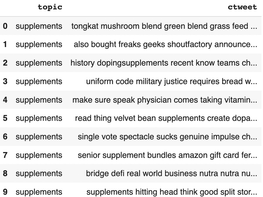
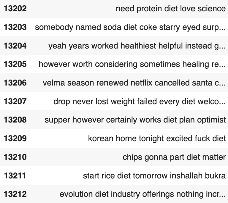
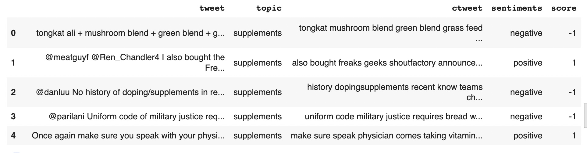
Cleaned dataset
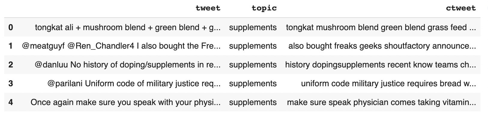
The dataset includes tweet data and the topics included
Training and Testing data
When building a machine learning model, it is important to divide the data into a training set and a testing set. The training set is used to train the model, while the testing set is used to evaluate its performance and generalization ability. In the context of supplement intake prediction using Naive Bayes, the data would be split into a training set and a testing set as follows: Data Split: The entire dataset containing information about individuals, their health status, and supplement intake would be randomly divided into two subsets: the training set and the testing set. Training Set: The training set would be used to train the Naive Bayes model by fitting the input features to the target variable (supplement intake). The model would learn from the input features in the training set and create a probabilistic model to predict the likelihood of supplement intake based on the input features. Testing Set: The testing set would be used to evaluate the performance of the Naive Bayes model. The model would predict the supplement intake for each individual in the testing set based on their input features. The predicted values would be compared to the actual supplement intake to measure the accuracy of the model. By splitting the data into a training set and a testing set, we can evaluate the performance of the Naive Bayes model and measure its ability to generalize to new data. The training set is used to fit the model parameters, while the testing set is used to evaluate the model's accuracy and generalization ability. The goal is to create a model that can accurately predict supplement intake for new individuals based on their input features.
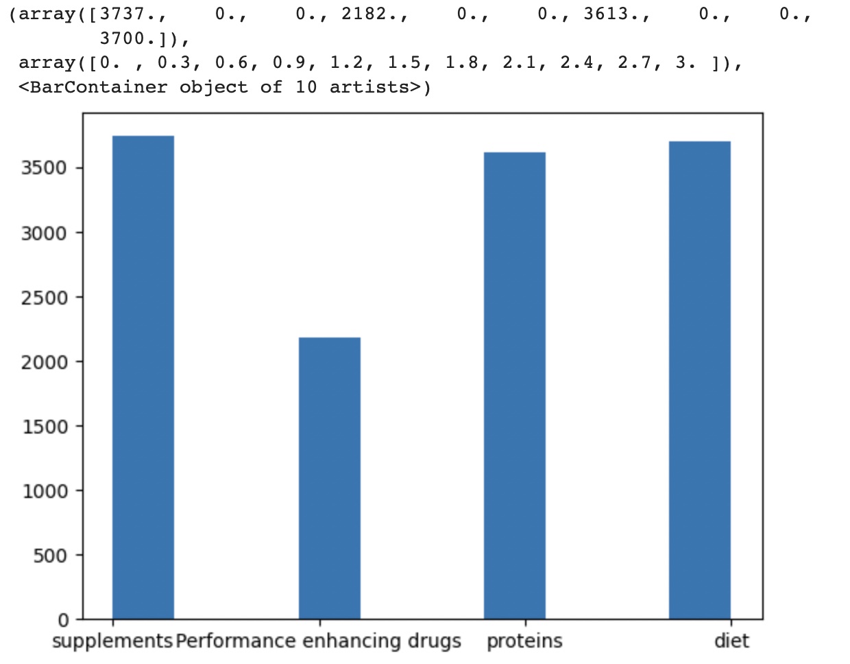
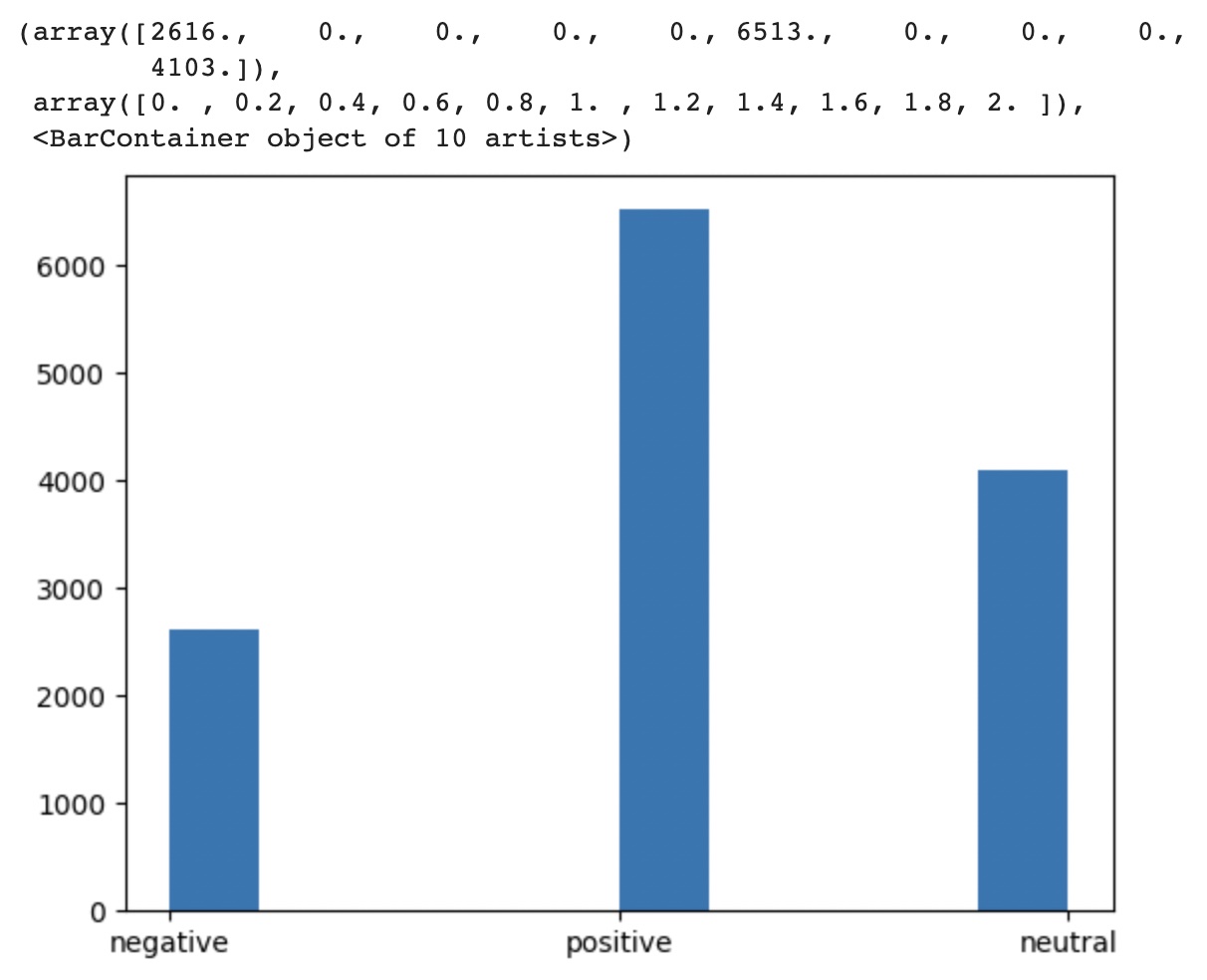
The data distribution for the given four topics and the sentiments associated with the tweetsfor all the topics extracted
Analysis
Standardizing data is an important step in neural network modeling to ensure that all input variables are on the same scale and to prevent any single variable from dominating the training process. Standardizing the values involves transforming the values of each variable to have zero mean and unit variance. Below is the transformed data
Analysis
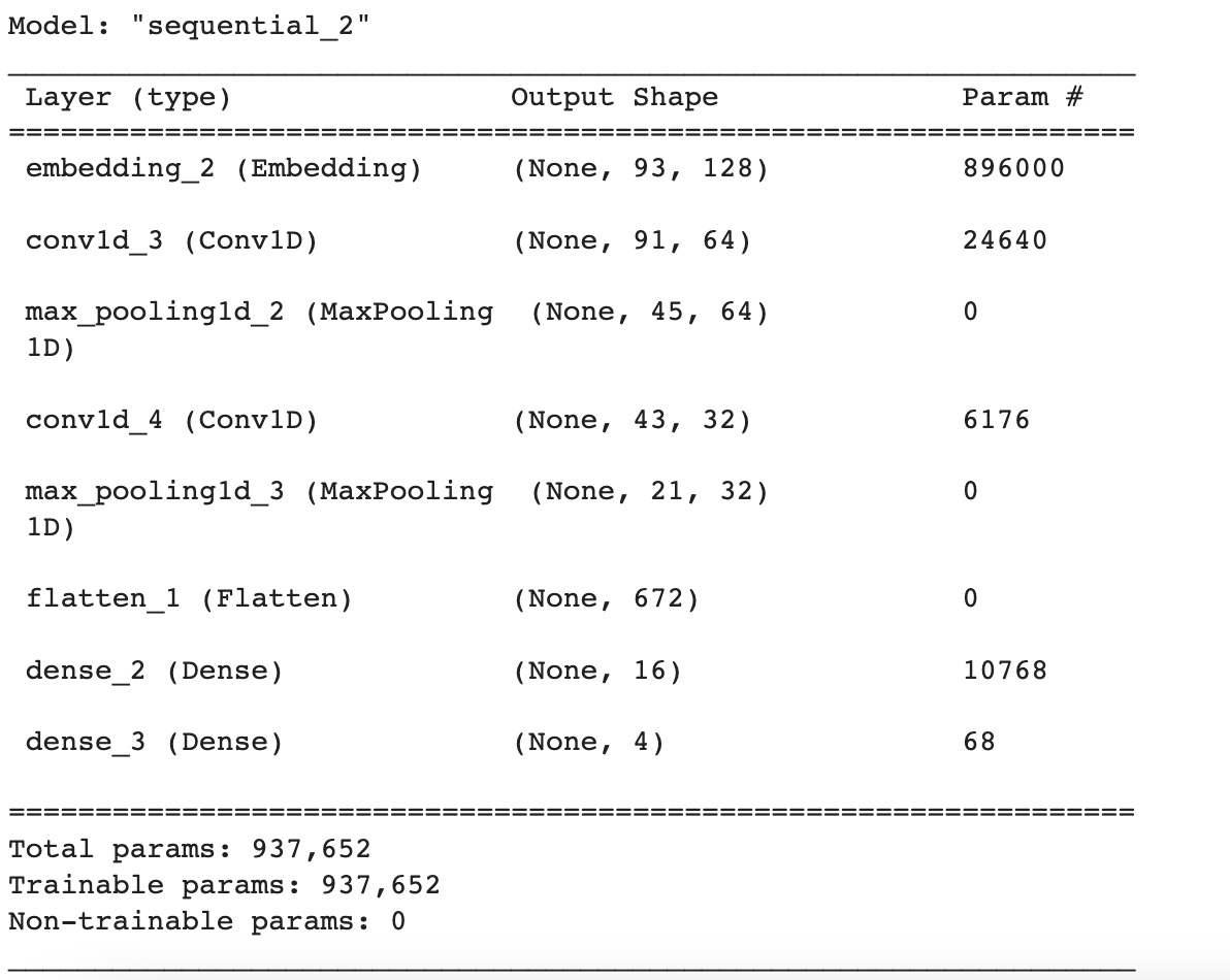
This is a Keras Sequential model with six layers: An Embedding layer with 896,000 trainable parameters, which maps integer word indices to dense vectors of size 128. A 1D Convolutional layer (Conv1D) with 24,640 trainable parameters, which applies 64 filters of size 3 to the input sequence. A MaxPooling1D layer (MaxPooling1D) with no trainable parameters, which downsamples the output of the previous layer by taking the maximum value over a window of size 2. Another Conv1D layer with 6,176 trainable parameters, which applies 32 filters of size 3 to the output of the previous layer. Another MaxPooling1D layer with no trainable parameters, which downsamples the output of the previous layer. A Flatten layer, which flattens the output of the previous layer into a 1D tensor. A Dense layer with 10,768 trainable parameters and ReLU activation, which computes a linear transformation of the input followed by a rectified linear activation function. A final Dense layer with 68 trainable parameters and softmax activation, which computes a linear transformation of the input followed by a softmax activation function that outputs a probability distribution over the four possible classes. The model has a total of 937,652 parameters, all of which are trainable. The first layer (Embedding) has the most parameters, followed by the first Conv1D layer.
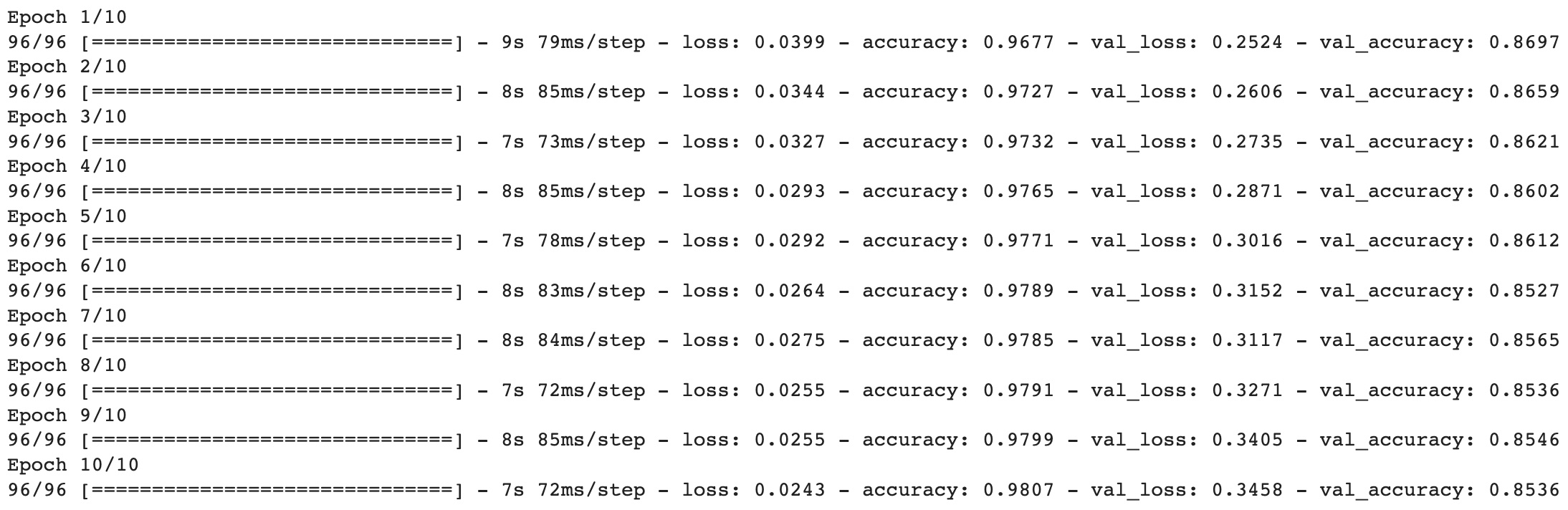
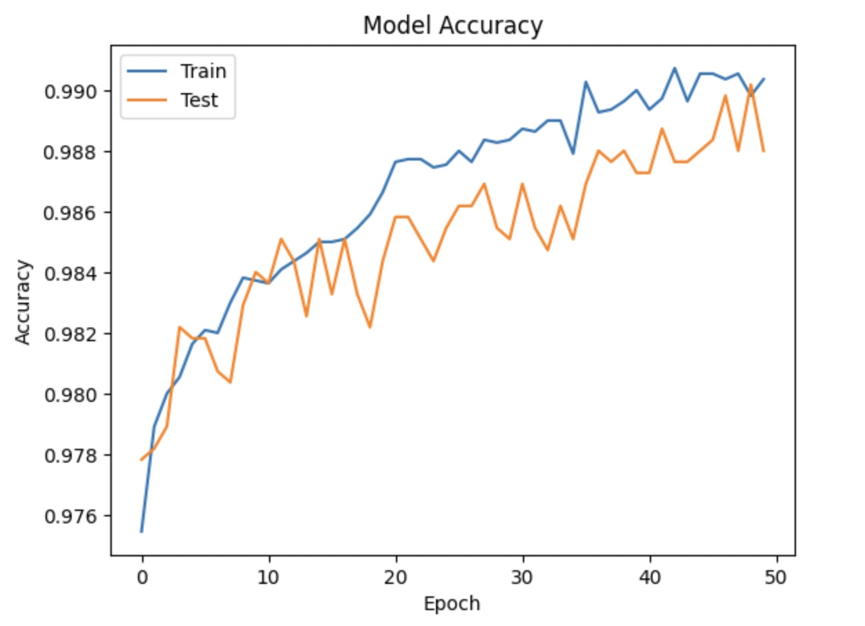
This is the output of a neural network model during training. The model is trained for 50 epochs, and this output shows the loss and accuracy metrics at each epoch. In each epoch, the model is fed with training data, which is used to update the weights of the model. The loss metric measures how well the model is predicting the output compared to the actual output. The accuracy metric measures the percentage of correct predictions made by the model. In the output shown, we can see that the loss value is decreasing and the accuracy value is increasing over the epochs. This is a good sign as it indicates that the model is improving in its predictions. By the end of the training, we can expect the loss value to be minimized and the accuracy value to be maximized.
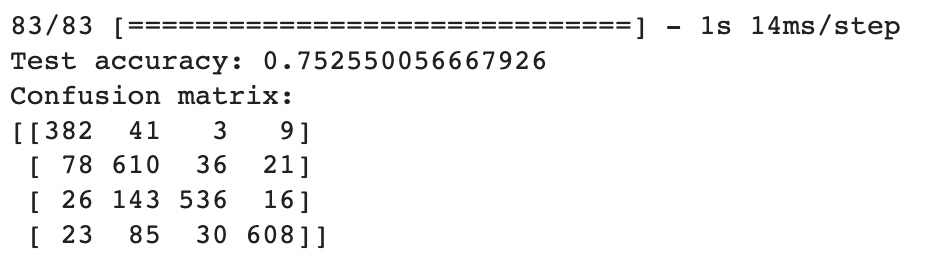
Accuracy score
The number 382 in the first row and first column means that 382 instances were correctly classified as protein, while 41 instances that actually belonged to the protein class were incorrectly classified as diet, 3 instances as drugs, and 9 instances as supplements. The diagonal elements of the matrix represent the instances that were correctly classified, while the off-diagonal elements represent the instances that were misclassified. The overall accuracy of the model can be calculated as the sum of the diagonal elements divided by the total number of instances. In this example, the model achieved an overall accuracy of 75%