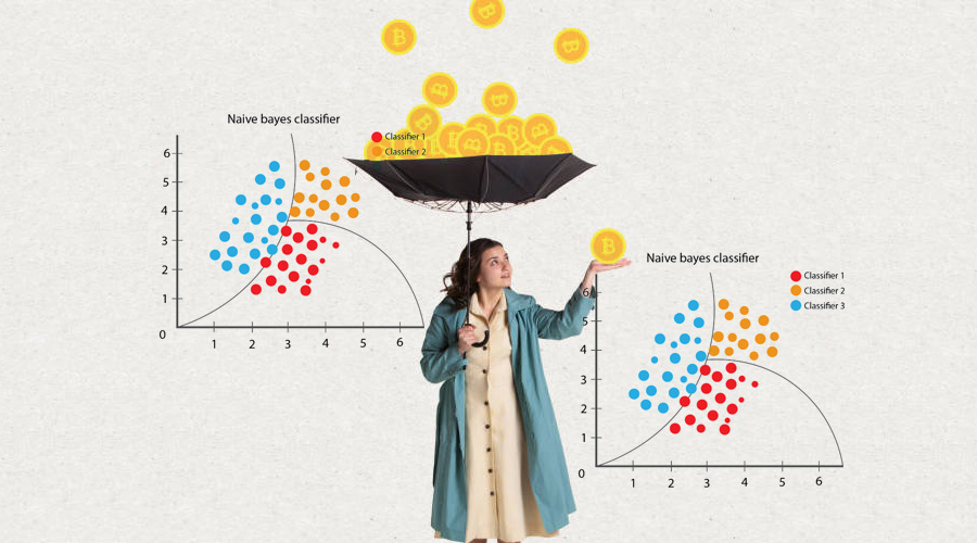
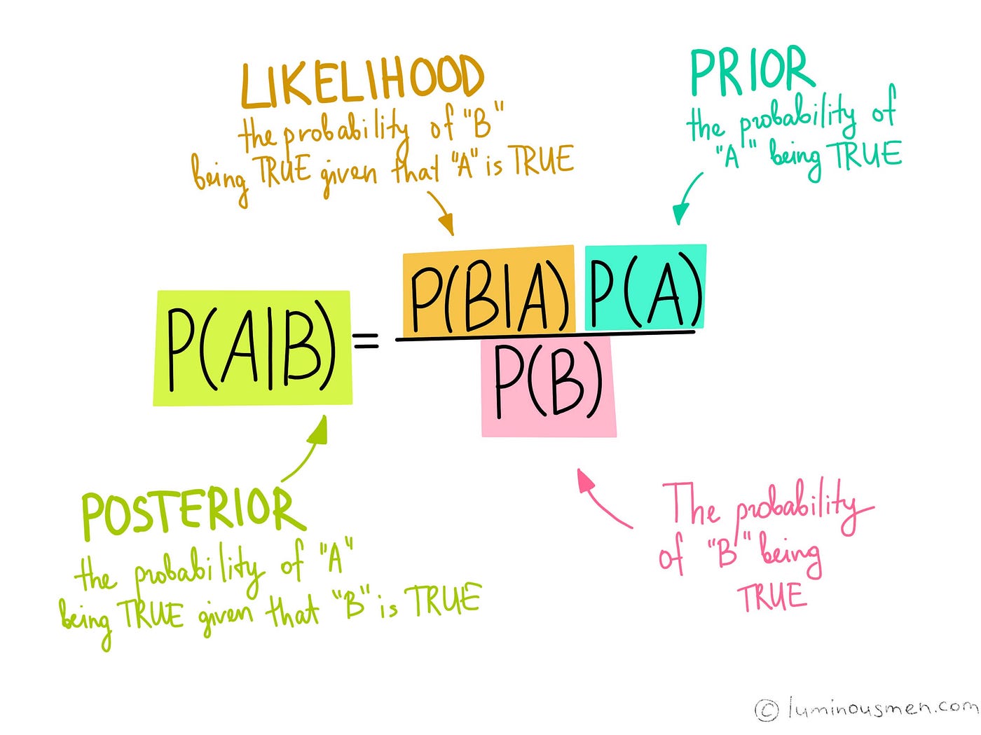
Naive Bayes (NB) is a classification algorithm based on Bayes' theorem, which is a fundamental theorem in probability theory. It is called "naive" because it makes a simplifying assumption that the features are conditionally independent of each other given the class label. This assumption simplifies the calculations required to estimate the probabilities involved in the algorithm and makes it computationally efficient. Naive Bayes works by calculating the probability of each class label given the observed feature vector. It does this by using Bayes' theorem, which states that the probability of a hypothesis (in this case, a class label) given some observed evidence is proportional to the product of the probability of the evidence given the hypothesis and the prior probability of the hypothesis.
Multinomial NB is a variant of NB that works with categorical data, such as text data, where the features represent the frequencies of occurrence of different words or tokens in a document. The algorithm models the probability of each word in the vocabulary given a particular class label, and then uses Bayes' theorem to calculate the probability of each class label given the observed feature vector.
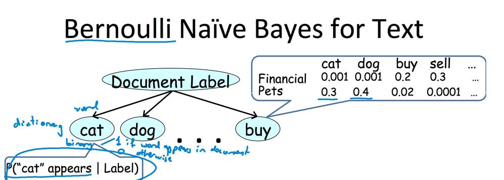
Bernoulli NB is another variant of NB that works with binary data, such as presence or absence of certain features in a document. In Bernoulli NB, the algorithm models the probability of each feature being present or absent given a particular class label, and then uses Bayes' theorem to calculate the probability of each class label given the observed feature vector. Both Multinomial and Bernoulli NB can be used for a variety of classification tasks, such as spam filtering, sentiment analysis, document classification, and more. They are particularly well-suited for text classification tasks, where the features are discrete and sparse, and the number of features can be very large. These algorithms are also very easy to implement and can perform well even with limited training data. However, their performance may suffer in cases where the independence assumption is not satisfied, or where the features are highly correlated with each other.
Used Clustering data: ClusterData_Twitter.csv
Link to the dataset: Dataset
Link to the Python code: Code
\
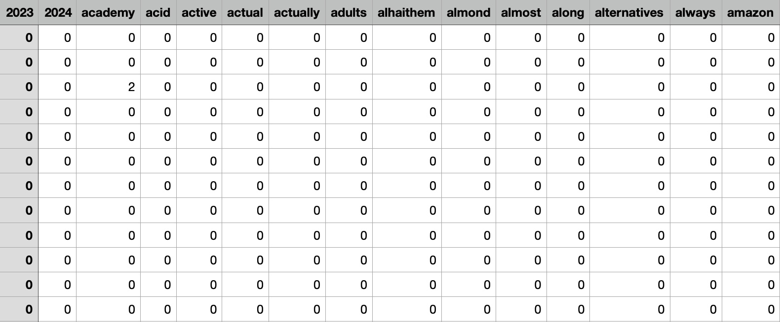
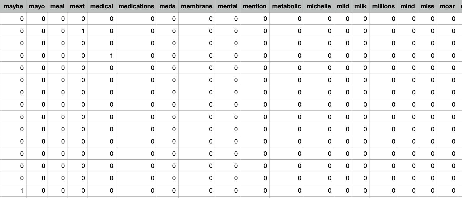
The dataset include numeric values of the count vectorized labels
Training and Testing data
When building a machine learning model, it is important to divide the data into a training set and a testing set. The training set is used to train the model, while the testing set is used to evaluate its performance and generalization ability.
In the context of supplement intake prediction using Naive Bayes, the data would be split into a training set and a testing set as follows: Data Split: The entire dataset containing information about individuals, their health status, and supplement intake would be randomly divided into two subsets: the training set and the testing set. Training Set: The training set would be used to train the Naive Bayes model by fitting the input features to the target variable (supplement intake). The model would learn from the input features in the training set and create a probabilistic model to predict the likelihood of supplement intake based on the input features. Testing Set: The testing set would be used to evaluate the performance of the Naive Bayes model. The model would predict the supplement intake for each individual in the testing set based on their input features. The predicted values would be compared to the actual supplement intake to measure the accuracy of the model. By splitting the data into a training set and a testing set, we can evaluate the performance of the Naive Bayes model and measure its ability to generalize to new data. The training set is used to fit the model parameters, while the testing set is used to evaluate the model's accuracy and generalization ability. The goal is to create a model that can accurately predict supplement intake for new individuals based on their input features.
Results
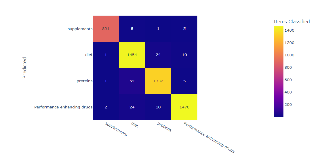
We load a dataset of supplement intake with labels, split the dataset into training and testing sets, apply Gaussian Naive Bayes classification, and evaluate its performance on the testing set. We calculate metrics such as accuracy, precision, recall, and F1 score to evaluate the performance of the Naive Bayes classifier, and print a confusion matrix to see the number of true positives, false positives, true negatives, and false negatives for each label. We can use these metrics to tune the hyperparameters of the Naive Bayes classifier and improve its performance on the task of classifying supplement intake with the labels diet, proteins, drugs, and supplements.
The results obtained from Naive Bayes classification may vary depending on the dataset and the specific hyperparameters chosen. In general, Naive Bayes classifiers are known for their simplicity, scalability, and ability to handle high-dimensional data. They often perform well on text classification tasks and can provide useful insights into the most important features for each class label. However, Naive Bayes classifiers make the "naive" assumption of feature independence, which may not hold true in some datasets. Additionally, Naive Bayes classifiers may suffer from the problem of class imbalance, where some classes have much fewer instances than others.
Accuracy score
An accuracy score of 94% means that the Naive Bayes classifier correctly classified 94% of the instances in the testing set. This is a good performance for the task of classifying supplement intake with the labels diet, proteins, drugs, and supplements. However, we should also consider other metrics such as precision, recall, and F1 score to evaluate the performance of the classifier more comprehensively. Additionally, we should examine the confusion matrix to see which classes the classifier is struggling to distinguish, and whether there are any patterns or biases in the misclassifications. Depending on the specific application, we may need to prioritize certain metrics over others. For example, in a medical diagnosis scenario, we may want to prioritize high recall (to minimize false negatives), while in a marketing campaign, we may want to prioritize high precision (to minimize false positives).
While a high accuracy score is generally desirable, it is important to consider other metrics such as precision, recall, and F1 score to get a more complete picture of the classifier's performance. For instance, if the dataset is imbalanced and one class has significantly fewer instances than the others, a high accuracy score may be misleading if the classifier simply predicts the majority class for most instances. In such cases, metrics such as precision and recall can provide more insights into the classifier's performance for each class label.